Examples
For usage examples with detailed descriptions take a look at the examples folder.
Basic usage
A simple usage example to find a path using the A* algorithm in a 3D environment.
Import the required libraries:
import numpy as np

from pathfinding3d.core.diagonal_movement import DiagonalMovement
from pathfinding3d.core.grid import Grid
from pathfinding3d.finder.a_star import AStarFinder
Create a Map:
Define a 3D grid using a numpy array. Any value smaller or equal to 0 represents an obstacle. Any positive value represents the weight of a field that can be walked on. The bigger the value higher the cost to walk that field. In this example, all walkable fields have the same cost of 1. Feel free to create a more complex map or use some sensor data as input for it.
# Define the 3D grid as 'x, y, z'
matrix = np.ones((3, 3, 3))
matrix[1, 1, 1] = 0  # Setting an obstacle at the center
Note: You can use different positive values to represent varying costs of traversing different fields.
Create the Grid:
Instantiate a Grid object from the map. This will create Node instances for every element of the map and also sets the size of the map.
grid = Grid(matrix=matrix)
Define Start and End Nodes:
Determine the start and end nodes on the grid. Coordinates start at 0. The nodes can be accessed by their coordinates. The first parameter is the x coordinate, the second the y coordinate and the third the z coordinate. So the top left corner is (0, 0, 0) and the bottom right corner is (2, 2, 2).
start = grid.node(0, 0, 0)
end = grid.node(2, 2, 2)
Instantiate the Pathfinding Finder:
Create a new instance of
AStarFinderand find the path. Here we allow diagonal movement which is not allowed by default. Thefind_pathmethod returns the path and the number of iterations needed.
finder = AStarFinder(diagonal_movement=DiagonalMovement.always)
path, runs = finder.find_path(start, end, grid)
Output the Result:
The path is a list with all the waypoints as nodes. Convert it to a list of coordinate tuples to pretty print it. Note that the start and end points are part of the path.
# Path will be a list with all the waypoints as nodes
# Convert it to a list of coordinate tuples
path = [p.identifier for p in path]

# Output the results
print("operations:", runs, "path length:", len(path))
print("path:", path)
Here is the whole example which you can copy-and-paste to play with it:
import numpy as np

from pathfinding3d.core.diagonal_movement import DiagonalMovement
from pathfinding3d.core.grid import Grid
from pathfinding3d.finder.a_star import AStarFinder

# Define the 3D grid
matrix = np.ones((3, 3, 3))
matrix[1, 1, 1] = 0
grid = Grid(matrix=matrix)

# Define start and end nodes
start = grid.node(0, 0, 0)
end = grid.node(2, 2, 2)

# Instantiate the finder and find the path
finder = AStarFinder(diagonal_movement=DiagonalMovement.always)
path, runs = finder.find_path(start, end, grid)

# Path will be a list with all the waypoints as nodes
# Convert it to a list of coordinate tuples
path = [p.identifier for p in path]

# Output the results
print("operations:", runs, "path length:", len(path))
print("path:", path)
Steps/Portals/Bridges
With pathfinding3d, you can seamlessly connect multiple grids. This feature is invaluable for simulating multi-story structures connected by staircases, bridges between different buildings, or even magical portals linking disparate locations.
Toy Example: Connecting Two Building Storeys with a Bridge
Let’s consider an example where we want to connect the second storey of two adjacent buildings with a bridge.
Define the Grids for Each Building:
Create two 3D grid arrays representing each building (‘world0’ and ‘world1’).
from pathfinding3d.core.grid import Grid
from pathfinding3d.core.world import World
from pathfinding3d.finder.a_star import AStarFinder

world0 = [[[1, 1, 1], [1, 0, 1], [1, 1, 1]],
          [[1, 1, 1], [1, 0, 1], [1, 1, 1]],
          [[1, 1, 1], [1, 0, 1], [1, 1, 1]]]
world1 = [[[1, 1, 1], [1, 0, 1], [1, 1, 1]],
          [[1, 1, 1], [1, 0, 1], [1, 1, 1]],
          [[1, 1, 1], [1, 0, 1], [1, 1, 1]]]
# create Grid instances for both worlds
grid0 = Grid(matrix=world0, grid_id=0)
grid1 = Grid(matrix=world1, grid_id=1)
Connect Nodes Between Grids:
Establish a two-way connection between nodes in different grids to simulate a bridge.
# connect the two worlds
grid0.node(2, 2, 2).connect(grid1.node(2, 2, 2))
grid1.node(2, 2, 2).connect(grid0.node(2, 2, 2))
Note: Establish connections in both directions for bi-directional travel. For unidirectional connections, define only one link.
Using the
Worldto Manage Multiple Grids:Create a
Worldobject to manage both grids, allowingfind_neighborsto access them during pathfinding.
# create a world instance
world = World({0: grid0, 1: grid1})
Pathfinding Across Connected Grids:
Utilize
AStarFinderto find a path from a start node in the first grid to an end node in the second grid. This time we need to pass theworldobject to thefind_pathmethod.
 # create a finder instance
 finder = AStarFinder()
 # find the path
 path, _ = finder.find_path(grid0.node(2, 0, 0), grid1.node(2, 0, 0), world)
This will output a path traversing from one building to another, demonstrating the unique capability of connecting different 3D spaces.
Visualizing the Path:
The path is a list of
Nodeobjects. We can convert the path to a list of tuples (x, y, z, grid_id) and separate the path into two lists of tuples (x, y, z) for each grid.
 # convert the path to a list of tuples (x, y, z, grid_id)
 path = [p.identifier for p in path]
 # separate the path into two lists of tuples (x, y, z)
 path0 = [p[:3] for p in path if p[3] == 0]
 path1 = [p[:3] for p in path if p[3] == 1]
 # print the paths
 print("path through world 0:", path0)
 print("path through world 1:", path1)
The output should look like this:
path through world 0: [(2, 0, 0), (2, 1, 0), (2, 2, 0), (2, 2, 1), (2, 2, 2)]
path through world 1: [(2, 2, 2), (2, 1, 2), (2, 0, 2), (2, 0, 1), (2, 0, 0)]
The path through world 0 starts at (2, 0, 0) and ends at (2, 2, 2). The path through world 1 starts at (2, 2, 2) and ends at (2, 0, 0). The two paths are connected by the bridge at (2, 2, 2).
Putting it all together:
from pathfinding3d.core.grid import Grid
from pathfinding3d.core.world import World
from pathfinding3d.finder.a_star import AStarFinder

world0 = [[[1, 1, 1], [1, 0, 1], [1, 1, 1]], [[1, 1, 1], [1, 0, 1], [1, 1, 1]], [[1, 1, 1], [1, 0, 1], [1, 1, 1]]]
world1 = [[[1, 1, 1], [1, 0, 1], [1, 1, 1]], [[1, 1, 1], [1, 0, 1], [1, 1, 1]], [[1, 1, 1], [1, 0, 1], [1, 1, 1]]]
# create Grid instances for both worlds
grid0 = Grid(matrix=world0, grid_id=0)
grid1 = Grid(matrix=world1, grid_id=1)

# connect the two worlds
grid0.node(2, 2, 2).connect(grid1.node(2, 2, 2))
grid1.node(2, 2, 2).connect(grid0.node(2, 2, 2))

# create a world instance
world = World({0: grid0, 1: grid1})

# create a finder instance
finder = AStarFinder()
# find the path
path, _ = finder.find_path(grid0.node(2, 0, 0), grid1.node(2, 0, 0), world)

# convert the path to a list of tuples (x, y, z, grid_id)
path = [p.identifier for p in path]
# separate the path into two lists of tuples (x, y, z)
path0 = [p[:3] for p in path if p[3] == 0]
path1 = [p[:3] for p in path if p[3] == 1]
# print the paths
print("path through world 0:", path0)
print("path through world 1:", path1)
Visualizing the Path
Sometimes it is helpful to visualize the path to better understand the algorithm. Here is a simple example using the open3d library for this purpose.
Prerequisites
Install the
open3dlibrary:pip install open3d
Example with Open3D
Import the required libraries:
import os

import numpy as np
import open3d as o3d

from pathfinding3d.core.diagonal_movement import DiagonalMovement
from pathfinding3d.core.grid import Grid
from pathfinding3d.finder.a_star import AStarFinder
Load the sample map:
# Load the map
matrix = np.load("sample_map.npy")
sample_map.npyis a numpy array of shape (42, 42, 42), where each element indicates an obstacle or free space. This file can be downloaded from the provided Github link.Create the Grid and define the start and end nodes:
# define start and end points as [x, y, z] coordinates
start_pt = [21, 21, 21]
end_pt = [5, 38, 33]

# create grid representation and start and end nodes
grid = Grid(matrix=matrix)
start = grid.node(*start_pt)
end = grid.node(*end_pt)
Note: The
*operator unpacks the list into individual arguments. Here, we define the start and end points of our path and create a grid representation of our 3D space.Find the path:
# initialize A* finder with specified diagonal movement setting
finder = AStarFinder(diagonal_movement=DiagonalMovement.only_when_no_obstacle)

# use the finder to get the path
path, runs = finder.find_path(start, end, grid)

# print results
path_cost = end.g
print(f"path cost: {path_cost:.4f}, path length: {len(path)}, runs: {runs}")
This will output:
path cost: 28.6130, path length: 20, runs: 458
The path cost can be accessed from the
endnode’sgattribute for A*.Visualize the path:
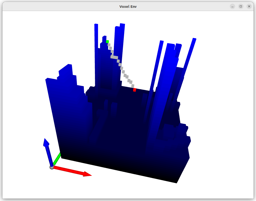
Find the obstacles and represent them in blue. The
colorsarray is a numpy array of shape (n, 3) where n is the number of obstacles. The first column represents the red channel, the second column represents the green channel, and the third column represents the blue channel. Thexyz_ptarray is a numpy array of shape (n, 3) where n is the number of obstacles. The first column represents the x coordinate, the second column represents the y coordinate, and the third column represents the z coordinate. Thexyz_ptarray is used to create aPointCloudobject which is then visualized usingdraw_geometries.# Identifying obstacles and representing them in blue obstacle_indices = np.where(matrix == 0) xyz_pt = np.stack(obstacle_indices, axis=-1).astype(float) colors = np.zeros((xyz_pt.shape[0], 3)) colors[:, 2] = obstacle_indices[2] / np.max(obstacle_indices[2])
The start point is represented in red and the end point is represented in green. The path is represented in grey.
path_colorsis a numpy array of shape (len(path) - 2, 3) where len(path) is the number of waypoints in the path. Since we already have the start and end points which are also part of the path, we subtract 2 from the length of the path to get the number of remaining waypoints.# Prepare start and end colors start_color = np.array([[1.0, 0, 0]]) # Red end_color = np.array([[0, 1.0, 0]]) # Green path_colors = np.full((len(path) - 2, 3), [0.7, 0.7, 0.7]) # Grey for the path
Now we can add the start and end points to the
xyz_ptarray along with the remaining waypoints in the path. Similarly the colors can be added to thecolorsarray. For every point in thexyz_ptarray, there is a corresponding color in thecolorsarray.# Combine points and colors for visualization xyz_pt = np.concatenate((xyz_pt, [start_pt], [end_pt], path[1:-1])) colors = np.concatenate((colors, start_color, end_color, path_colors))
Create a
PointCloudobject with thexyz_ptandcolorsarrays.# Create the point cloud pcd = o3d.geometry.PointCloud() pcd.points = o3d.utility.Vector3dVector(xyz_pt) pcd.colors = o3d.utility.Vector3dVector(colors)
Create a
VoxelGridobject from thePointCloudobject. This will generate a voxel grid from the point cloud. Thevoxel_sizeparameter determines the size of the voxels.# Create the voxel grid from the point cloud voxel_grid = o3d.geometry.VoxelGrid.create_from_point_cloud(pcd, voxel_size=1.0) axes = o3d.geometry.TriangleMesh.create_coordinate_frame(size=15.0, origin=np.array([-3.0, -3.0, -3.0]))
The axes is for reference and can be removed if not needed.
Visualize the voxel grid. The
widthandheightparameters determine the size of the window.# Visualize the voxel grid o3d.visualization.draw_geometries([axes, voxel_grid], window_name="Voxel Env", width=1024, height=768)
You can rotate the voxel grid by clicking and dragging the mouse. You can also zoom in and out using the mouse wheel.
The output should look like this:
The full code is available here: 03_view_map
Example with any angle of movement
Often, it is desirable to allow movement in any direction rather than being restricted to the 26 discrete directions in a 3D grid. This can be achieved by using the ThetaStarFinder class. The ThetaStarFinder class is a subclass of the AStarFinder class and can be used in the same way.
Let’s cut to the chase and see how it works:
As usual, import the required libraries:
import numpy as np

from pathfinding3d.core.grid import Grid
from pathfinding3d.finder.theta_star import ThetaStarFinder
For this example, we will use a simple 3D grid with a single obstacle in the middle. The start point is at the bottom left corner and the end point is at the top right corner.
# Define the 3D grid
matrix = np.ones((10, 10, 10), dtype=np.int8)
matrix[5, 5, 5] = 0  # Setting an obstacle at the center

# Create the grid representation
grid = Grid(matrix=matrix)

# Define start and end points
start = grid.node(0, 0, 0) # Bottom left corner
end = grid.node(9, 9, 9) # Top right corner
Instantiate the
ThetaStarFinderclass and find the path:# Instantiate the finder finder = ThetaStarFinder() path, runs = finder.find_path(start, end, grid) # Convert the path to a list of coordinate tuples path = [p.identifier for p in path]
Note: The
ThetaStarFinderwill always have diagonal movements enabled.Output the results:
# Output the results
print("operations:", runs, "path length:", len(path))
print("path:", path)
This will output:
operations: 12 path length: 3
path: [(0, 0, 0), (9, 8, 8), (9, 9, 9)]
You will notice that the path does not have all the waypoints as other algorithms. This is because the
ThetaStarFinderalgorithm will smooth the path by checking whether there is a direct path between two waypoints (Line of Sight). If there is a direct path, the intermediate waypoints are removed. This is useful for applications where the path needs to be traversed by a vehicle. The vehicle can move in any direction and does not need to follow a grid. The path can be smoothed to reduce the number of waypoints to be traversed.For a quantitative analysis let’s compare the number of waypoints in the path for the
AStarFinderandThetaStarFinderalgorithms:from pathfinding3d.finder.a_star import AStarFinder # Instantiate the finder finder = AStarFinder() # Cleanup the grid grid.cleanup() # Find the path using AStarFinder astar_path, runs = finder.find_path(start, end, grid) # Convert the path to a list of coordinate tuples astar_path = [p.identifier for p in astar_path] print("AStarFinder operations:", runs, "AStarFinder path length:", len(path)) print("AStarFinder path:", path)
This will output:
AStarFinder operations: 52 AStarFinder path length: 11
AStarFinder path: [(0, 0, 0), (1, 1, 1), (2, 2, 2), (3, 3, 3), (4, 4, 4), (5, 4, 4), (6, 5, 5), (7, 6, 6), (8, 7, 7), (9, 8, 8), (9, 9, 9)]
As you can see, the
AStarFinderalgorithm has 11 waypoints in the path. Let’s compare the cost of the path for both algorithms:# Function to calculate the cost of the path def calculate_path_cost(path): cost = 0 for pt, pt_next in zip(path[:-1], path[1:]): dx, dy, dz = pt_next[0] - pt[0], pt_next[1] - pt[1], pt_next[2] - pt[2] cost += (dx**2 + dy**2 + dz**2) ** 0.5 return cost # Calculate the cost of the path for ThetaStarFinder theta_star_cost = calculate_path_cost(path) # Calculate the cost of the path for AStarFinder astar_cost = calculate_path_cost(astar_path) # Output the results print("ThetaStarFinder path cost:", theta_star_cost, "\nAStarFinder path cost:", astar_cost)
This will output:
ThetaStarFinder path cost: 15.871045857174057
AStarFinder path cost: 16.27062002292411
As you can see, the
ThetaStarFinderalgorithm has a lower cost than theAStarFinderalgorithm. Thus theThetaStarFinderalgorithm can be more efficient for applications with any angle of movement.We can visualize the paths using
plotlythis time:import plotly.graph_objects as go # Create a plotly figure to visualize the path fig = go.Figure( data=[ go.Scatter3d( x=[pt[0] + 0.5 for pt in path], y=[pt[1] + 0.5 for pt in path], z=[pt[2] + 0.5 for pt in path], mode="lines + markers", line=dict(color="blue", width=4), marker=dict(size=4, color="blue"), name="Theta* path", hovertext=["Theta* path point"] * len(path), ), go.Scatter3d( x=[pt[0] + 0.5 for pt in astar_path], y=[pt[1] + 0.5 for pt in astar_path], z=[pt[2] + 0.5 for pt in astar_path], mode="lines + markers", line=dict(color="red", width=4), marker=dict(size=4, color="red"), name="A* path", hovertext=["A* path point"] * len(astar_path), ), go.Scatter3d( x=[5.5], y=[5.5], z=[5.5], mode="markers", marker=dict(color="black", size=7.5), name="Obstacle", hovertext=["Obstacle point"], ), go.Scatter3d( x=[0.5], y=[0.5], z=[0.5], mode="markers", marker=dict(color="green", size=7.5), name="Start", hovertext=["Start point"], ), go.Scatter3d( x=[9.5], y=[9.5], z=[9.5], mode="markers", marker=dict(color="orange", size=7.5), name="End", hovertext=["End point"], ), ] ) # Define the camera position camera = { "up": {"x": 0, "y": 0, "z": 1}, "center": {"x": 0.1479269806756467, "y": 0.06501594452841505, "z": -0.0907033779622012}, "eye": {"x": 1.3097359159706334, "y": 0.4710974884501846, "z": 2.095154166796815}, "projection": {"type": "perspective"}, } # Update the layout of the figure fig.update_layout( scene=dict( xaxis=dict( title="x - axis", backgroundcolor="white", gridcolor="lightgrey", showbackground=True, zerolinecolor="white", range=[0, 10], dtick=1, ), yaxis=dict( title="y - axis", backgroundcolor="white", gridcolor="lightgrey", showbackground=True, zerolinecolor="white", range=[0, 10], dtick=1, ), zaxis=dict( title="z - axis", backgroundcolor="white", gridcolor="lightgrey", showbackground=True, zerolinecolor="white", range=[0, 10], dtick=1, ), ), legend=dict( yanchor="top", y=0.99, xanchor="left", x=0.01, bgcolor="rgba(255, 255, 255, 0.7)", ), title=dict(text="Theta* vs A*"), scene_camera=camera, ) # Show the figure in a new tab fig.show()
This will open a new tab in your browser with the following visualization:
You can rotate the figure by clicking and dragging the mouse. You can also zoom in and out using the mouse wheel.
The full code is available here: 04_theta_star.